正所谓前人栽树,后人乘凉。
感谢To_2019_1_4提供的非常详尽的资料。
安装R和Bioconductor包
$ sudo apt-get install r-base-core libxml2-dev libcurl4-openssl-dev curl
$ R
之后在R环境中安装Bioconductor包
> # 加载Bioconductor的安装脚本
> source("http://bioconductor.org/biocLite.R")
> # 安装Bioconductor的核心包
> biocLite()
> # 安装GEO包
> biocLite("GEOquery")
下载芯片数据
本文以GSE20986为例。首选我们从GEO数据库下载原始数据,导入GEOquery包,用它下载原始数据:
> library(GEOquery)
> getGEOSuppFiles("gse10986") 下载完成后,打开文件管理器,在启动 R 程序的文件夹里可以看到当前文件夹下生成了一个 GSE20986 文件夹,可以直接查看文件夹里的内容:

> $ ls GSE20986/
filelist.txt GSE20986_RAW.tar GSE20986_RAW.tar 文件是压缩打包的 CEL(Affymetrix array 数据原始格式)文件。先解包数据,再解压数据。这些操作可以直接在 R 命令终端中进行:

> untar("GSE20986/GSE20986_RAW.tar", exdir="data")
> cels <- list.files("data/", pattern = "[gz]")
> sapply(paste("data", cels, sep="/"), gunzip)
> cels # 芯片实验信息整理 在对数据进行分析之前,我们需要先整理好实验设计信息。这其实就是一个文本文件,包含芯片名字、此芯片上杂交的样本名字。为了方便在 R 中 使用 simpleaffy 包读取实验信息文本文件,需要先编辑好格式:

$ ls -1 data/*.CEL > data/phenodata.txt 将这个文本文件用编辑器打开,现在其中只有一列 CEL 文件名,最终的实验信息文本需要包含三列数据(用 tab 分隔),分别是 Name, FileName, Target。本教程中 Name 和 FileName 这两栏是相同的,当然 Name 这一栏可以用更加容易理解的名字代替。
Target 这一栏数据是芯片上的样本标签,例如 iris, retina, HUVEC, choroidal,这些标签定义了那些数据是生物学重复以便后面的分析。
这个实验信息文本文件最终格式是这样的:
Name FileName Target
GSM524662.CEL GSM524662.CEL iris
GSM524663.CEL GSM524663.CEL retina
GSM524664.CEL GSM524664.CEL retina
GSM524665.CEL GSM524665.CEL iris
GSM524666.CEL GSM524666.CEL retina
GSM524667.CEL GSM524667.CEL iris
GSM524668.CEL GSM524668.CEL choroid
GSM524669.CEL GSM524669.CEL choroid
GSM524670.CEL GSM524670.CEL choroid
GSM524671.CEL GSM524671.CEL huvec
GSM524672.CEL GSM524672.CEL huvec
GSM524673.CEL GSM524673.CEL huvec 注意:每栏之间是使用 Tab 进行分隔的,而不是空格! # 载入数据并对其进行标准化 需要先安装 simpleaffy 包,simpleaffy 包提供了处理 CEL 数据的程序,可以对 CEL 数据进行标准化同时导入实验信息(即前一步中整理好的实验信息文本文件内容),导入数据到 R 变量 celfiles 中:
> biocLite("simpleaffy")
> library(simpleaffy)
> celfiles <- read.affy(covdesc="phenodata.txt", path="data") 你可以通过输入 ‘celfiles’ 来确定数据导入成功并添加芯片注释(第一次输入 ‘celfiles’ 的时候会进行注释):
> celfiles
AffyBatch object
size of arrays=1164x1164 features (12 kb)
cdf=HG-U133_Plus_2 (54675 affyids)
number of samples=12
number of genes=54675
annotation=hgu133plus2
notes= 现在我们需要对数据进行标准化,使用 GC-RMA 算法对 GEO 数据库中的数据进行标准化,第一次运行的时候需要下载一些其他的必要文件:
> celfiles.gcrma <- gcrma(celfiles)
Adjusting for optical effect............Done.
Computing affinitiesLoading required package: AnnotationDbi
.Done.
Adjusting for non-specific binding............Done.
Normalizing
Calculating Expression 如果你想看标准化之后的数据,输入 celfiles.gcrma, 你会发现提示已经不是 AffyBatch object 了,而是 ExpressionSet object,是已经标准化了的数据:
> celfiles.gcrma
ExpressionSet (storageMode: lockedEnvironment)
assayData: 54675 features, 12 samples
element names: exprs
protocolData
sampleNames: GSM524662.CEL GSM524663.CEL ... GSM524673.CEL (12 total)
varLabels: ScanDate
varMetadata: labelDescription
phenoData
sampleNames: GSM524662.CEL GSM524663.CEL ... GSM524673.CEL (12 total)
varLabels: sample FileName Target
varMetadata: labelDescription
featureData: none
experimentData: use 'experimentData(object)'
Annotation: hgu133plus2 # 数据质量控制 再进行下一步的数据分析之前,我们有必要对数据质量进行检查,确保没有其他的问题。首先,可以通过对标准化之前和之后的数据画箱线图来检查 GC-RMA 标准化的效果:
> # 载入色彩包
> library(RColorBrewer)
> # 设置调色板
> cols <- brewer.pal(8, "Set1")
> # 对标准化之前的探针信号强度做箱线图
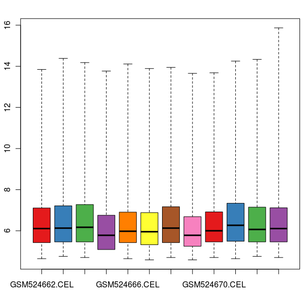
> boxplot(celfiles, col=cols)
> # 对标准化之后的探针信号强度做箱线图,需要先安装 affyPLM 包,以便解析 celfiles.gcrma 数据
> biocLite("affyPLM")
> library(affyPLM)
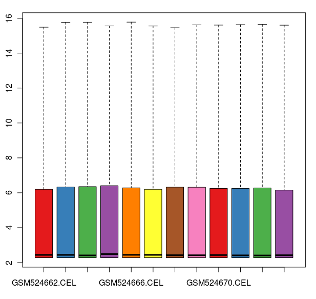
> boxplot(celfiles.gcrma, col=cols)
> # 标准化前后的箱线图会有些变化
> # 但是密度曲线图看起来更直观一些
> # 对标准化之前的数据做密度曲线图
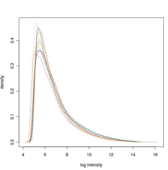
> hist(celfiles, col=cols)
> # 对标准化之后的数据做密度曲线图
> hist(celfiles.gcrma, col=cols) 数据标准化之前的箱线图
数据标准化之后的箱线图
数据标准化之前的密度曲线图
数据标准化之后的密度曲线图
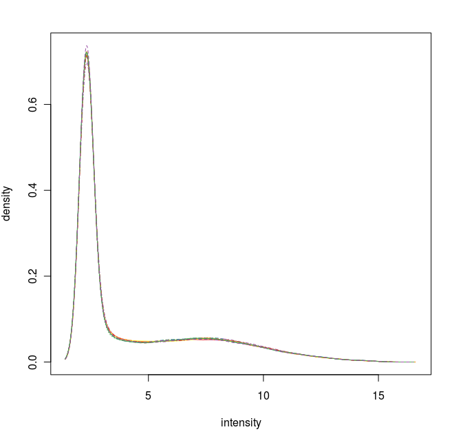
通过这些图我们可以看出这12张芯片数据之间差异不大,标准化处理将所有芯片信号强度标准化到具有类似分布特征的区间内。为了更详细地了解芯片探针信号强度,我们可以使用 affyPLM 对单个芯片 CEL 数据进行可视化。
> # 从 CEL 文件读取探针信号强度(fitPLM 功能:通过拟合探针水平模型(probe-level model),将AffyBatch转换为PLMset):
> celfiles.qc <- fitPLM(celfiles)
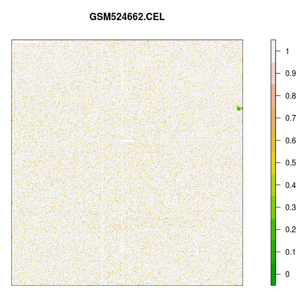
> # 对芯片 GSM24662.CEL 信号进行可视化:
> image(celfiles.qc, which=1, add.legend=TRUE)
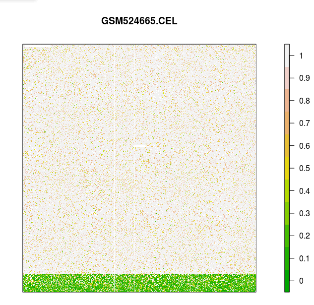
> # 对芯片 GSM524665.CEL 进行可视化
> # 这张芯片数据有些人为误差
> image(celfiles.qc, which=4, add.legend=TRUE)
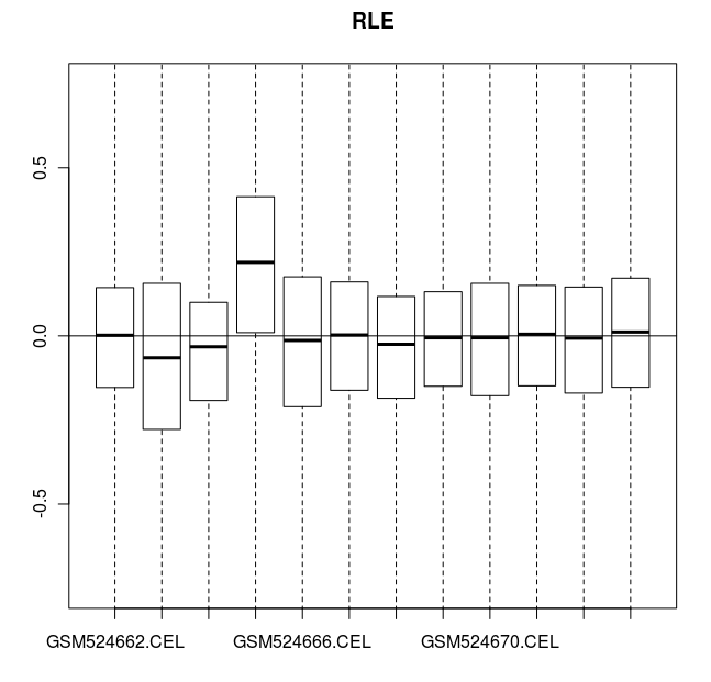
> # affyPLM 包还可以画箱线图
> # RLE (Relative Log Expression 相对表达量取对数) 图中
> # 所有的值都应该接近于零。 GSM524665.CEL 芯片数据由于有人为误差而例外。
> RLE(celfiles.qc, main="RLE")
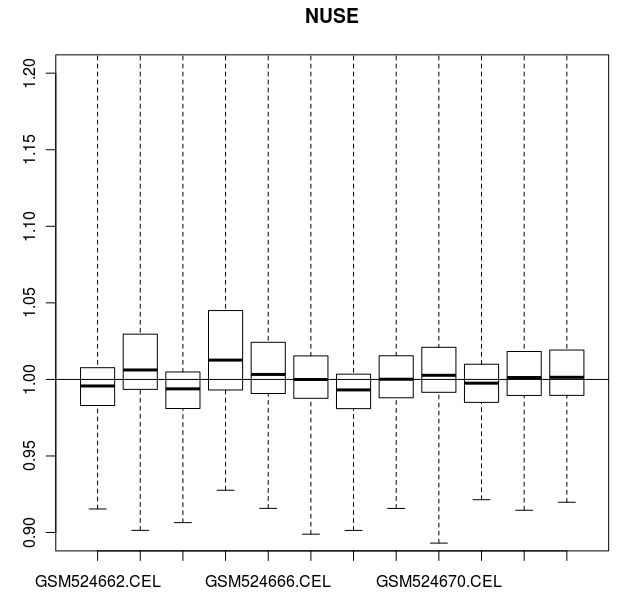
> # 也可以用 NUSE (Normalised Unscaled Standard Errors)作图比较.
> # 对于绝大部分基因,标准差的中位数应该是1。
> # 芯片 GSM524665.CEL 在这个图中,同样是一个例外
> NUSE(celfiles.qc, main="NUSE")
标准的芯片 AffyPLM 信号图
存在人工误差的芯片 AffyPLM 信号图
CEL 数据的 RLE 图
CEL 数据的 NUSE 图
我们还可以通过层次聚类来查看样本之间的关系:
> eset <- exprs(celfiles.gcrma)
> distance <- dist(t(eset),method="maximum")
> clusters <- hclust(distance)
> plot(clusters) 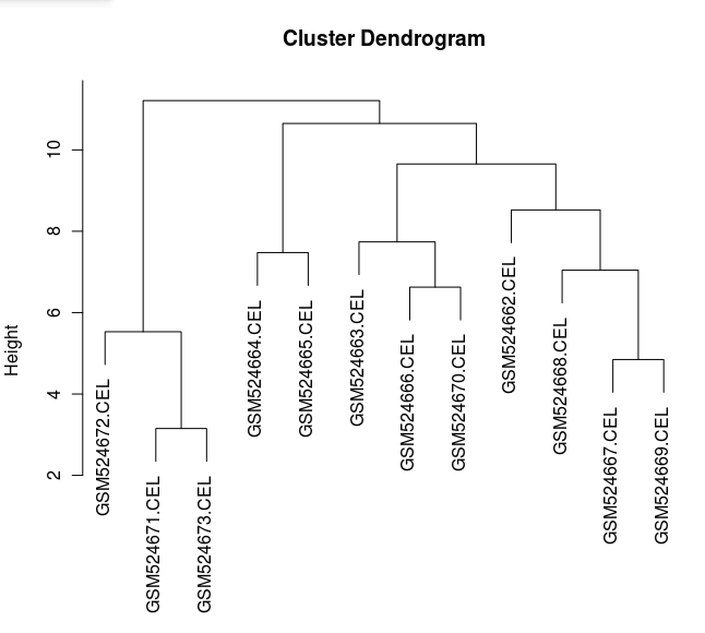
图形显示,与其他眼组织相比 HUVEC 样品是单独的一组,表现出组织类型聚集的一些特征,另外 GSM524665.CEL 数据在此图中并不显示为异常值。
数据过滤
现在我们可以对数据进行分析了,分析的第一步就是要过滤掉数据中的无用数据,例如作为内参的探针数据,基因表达无明显变化的数据(在差异表达统计时也会被过滤掉),信号值与背景信号差不多的探针数据。 下面的 nsFilter 参数是为了不删除没有 Entrez Gene ID 的位点,保留有重复 Entrez Gene ID 的位点:
> celfiles.filtered <- nsFilter(celfiles.gcrma, require.entrez=FALSE, remove.dupEntrez=FALSE)
> # 哪些位点被过滤掉了?为什么?
> celfiles.filtered$filter.log
$numLowVar
[1] 27307

$feature.exclude
[1] 62
我们可以看出有 27307 个探针位点因为无明显表达差异(LowVar)被过滤掉,有 62 个探针位点因为是内参而被过滤掉。
查找有表达差异的探针位点
现在有了过滤之后的数据,我们就可以用 limma 包进行差异表达分析了。首先,我们要提取样本的信息:
> samples <- celfiles.gcrma$Target
> # 检查数据的分组信息
> samples
[1] "iris" "retina" "retina" "iris" "retina" "iris" "choroid"
[8] "choroid" "choroid" "huvec" "huvec" "huvec"
> # 将分组数据转换为因子类型变量
> samples <- as.factor(samples)
> # 检查转换的因子变量
> samples
[1] iris retina retina iris retina iris choroid choroid choroid
[10] huvec huvec huvec
Levels: choroid huvec iris retina
> # 设置实验分组,请见:https://github.com/bioconductor-china/basic/blob/master/makeContrasts.md
> design <- model.matrix(~0 + samples)
> colnames(design) <- c("choroid", "huvec", "iris", "retina")
> # 检查实验分组
> design
choroid huvec iris retina
1 0 0 1 0
2 0 0 0 1
3 0 0 0 1
4 0 0 1 0
5 0 0 0 1
6 0 0 1 0
7 1 0 0 0
8 1 0 0 0
9 1 0 0 0
10 0 1 0 0
11 0 1 0 0
12 0 1 0 0
attr(,"assign")
[1] 1 1 1 1
attr(,"contrasts")
attr(,"contrasts")$samples
[1] "contr.treatment"
现在我们将芯片数据进行了标准化和过滤,也有样品分组和实验分组信息,可以将数据导入 limma 包进行差异表达分析了:
> library(limma)
> # 将线性模型拟合到过滤之后的表达数据集上
> fit <- lmFit(exprs(celfiles.filtered$eset), design)
> # 建立对比矩阵以比较组织和细胞系
> contrast.matrix <- makeContrasts(huvec_choroid = huvec - choroid, huvec_retina = huvec - retina, huvec_iris <- huvec - iris, levels=design)
> # 检查对比矩阵
> contrast.matrix
Contrasts
Levels huvec_choroid huvec_retina huvec_iris
choroid -1 0 0
huvec 1 1 1
iris 0 0 -1
retina 0 -1 0
> # 现在将对比矩阵与线性模型拟合,比较不同细胞系的表达数据
> huvec_fits <- contrasts.fit(fit, contrast.matrix)
> # 使用经验贝叶斯算法计算差异表达基因的显著性
> huvec_ebFit <- eBayes(huvec_fits)
> # 返回对应比对矩阵 top 10 的结果
> # coef=1 是 huvec_choroid 比对矩阵, coef=2 是 huvec_retina 比对矩阵
> topTable(huvec_ebFit, number=10, coef=1)
ID logFC AveExpr t P.Value adj.P.Val
6147 204779_s_at 7.367947 4.171874 72.77016 3.290669e-15 8.985500e-11
7292 207016_s_at 6.934796 4.027229 57.37259 3.712060e-14 5.068076e-10
8741 209631_s_at 5.193313 4.003541 51.22423 1.177337e-13 1.071612e-09
26309 242809_at 6.433514 4.167462 48.52518 2.042404e-13 1.394247e-09
6828 205893_at 4.480463 3.544350 40.59376 1.253534e-12 6.845801e-09
20232 227377_at 3.670688 3.209217 36.03427 4.200854e-12 1.911809e-08
6222 204882_at -5.351976 6.512018 -34.70239 6.154318e-12 2.400711e-08
27051 38149_at -5.051906 6.482418 -31.44098 1.672263e-11 5.282592e-08
6663 205576_at 6.586372 4.139236 31.31584 1.741131e-11 5.282592e-08
6589 205453_at 3.623706 3.210306 30.72793 2.109110e-11 5.759136e-08
B
6147 20.25563
7292 19.44681
8741 18.96282
26309 18.70767
6828 17.75331
20232 17.01960
6222 16.77196
27051 16.08854
6663 16.05990
6589 15.92277
分析结果的各列数据含义:
第一列是探针组在表达矩阵中的行号;
第二列“ID” 是探针组的 AffymatrixID;
第三列“logFC”是两组表达值之间以2为底对数化的的变化倍数(Fold change, FC)由于基因表达矩阵本身已经取了对数,这里实际上只是两组基因表达值均值之差;
第四列“AveExpr”是该探针组所在所有样品中的平均表达值;
第五列“t”是贝叶斯调整后的两组表达值间 T 检验中的 t 值;
第六列“P.Value”是贝叶斯检验得到的 P 值;
第七列“adj.P.Val”是调整后的 P 值;
第八列“B”是经验贝叶斯得到的标准差的对数化值。
如果要设置一个倍数变化阈值,并查看不同阈值返回了多少基因,可以使用 topTable 的 lfc 参数,参数设置为 5,4,3,2 时返回的基因个数:
> nrow(topTable(huvec_ebFit, coef=1, number=10000, lfc=5))
[1] 88
> nrow(topTable(huvec_ebFit, coef=1, number=10000, lfc=4))
[1] 194
> nrow(topTable(huvec_ebFit, coef=1, number=10000, lfc=3))
[1] 386
> nrow(topTable(huvec_ebFit, coef=1, number=10000, lfc=2))
[1] 1016
> # 提取表达量倍数变化超过 4 的探针列表
> probeset.list <- topTable(huvec_ebFit, coef=1, number=10000, lfc=4)
注释差异分析结果的基因 ID
为了将探针集注释上基因 ID 我们需要先安装一些数据库的包和注释的包,之后可以提取 topTable 中的探针 ID 并注释上基因 ID:
> biocLite("hgu133plus2.db")
> library(hgu133plus2.db)
> library(annotate)
> gene.symbols <- getSYMBOL(probeset.list$ID, "hgu133plus2")
> results <- cbind(probeset.list, gene.symbols)
> head(results)
ID logFC AveExpr t P.Value adj.P.Val
6147 204779_s_at 7.367947 4.171874 72.77016 3.290669e-15 8.985500e-11
7292 207016_s_at 6.934796 4.027229 57.37259 3.712060e-14 5.068076e-10
8741 209631_s_at 5.193313 4.003541 51.22423 1.177337e-13 1.071612e-09
26309 242809_at 6.433514 4.167462 48.52518 2.042404e-13 1.394247e-09
6828 205893_at 4.480463 3.544350 40.59376 1.253534e-12 6.845801e-09
6222 204882_at -5.351976 6.512018 -34.70239 6.154318e-12 2.400711e-08
B gene.symbols
6147 20.25563 HOXB7
7292 19.44681 ALDH1A2
8741 18.96282 GPR37
26309 18.70767 IL1RL1
6828 17.75331 NLGN1
6222 16.77196 ARHGAP25
> write.table(results, "results.txt", sep="\t", quote=FALSE)
还有后续的 Simon Cockell 的分析差异表达的生物学意义教程,即 GO,kegg 等注释,以及 Colin Gillespie 的差异表达分析可视化之火山图教程。
最后附上教程中的代码,请在确保你的文件夹中有已经编辑好的 phenodata.txt 文件之后再运行:
> # download the BioC installation routines
> source("http://bioconductor.org/biocLite.R")
> # install the core packages
> biocLite()
> # install the GEO libraries
> biocLite("GEOquery")
> library(GEOquery)
> getGEOSuppFiles("GSE20986")
> untar("GSE20986/GSE20986_RAW.tar", exdir="data")
> cels <- list.files("data/", pattern = "[gz]")
> sapply(paste("data", cels, sep="/"), gunzip)
> cels
> library(simpleaffy)
> celfiles<-read.affy(covdesc="phenodata.txt", path="data")
> celfiles
> celfiles.gcrma<-gcrma(celfiles)
> celfiles.gcrma
> # load colour libraries
> library(RColorBrewer)
> # set colour palette
> cols <- brewer.pal(8, "Set1")
> # plot a boxplot of unnormalised intensity values
> boxplot(celfiles, col=cols)
> # plot a boxplot of normalised intensity values, affyPLM required to interrogate celfiles.gcrma
> library(affyPLM)
> boxplot(celfiles.gcrma, col=cols)
> # the boxplots are somewhat skewed by the normalisation algorithm
> # and it is often more informative to look at density plots
> # Plot a density vs log intensity histogram for the unnormalised data
> hist(celfiles, col=cols)
> # Plot a density vs log intensity histogram for the normalised data
> hist(celfiles.gcrma, col=cols)
> # Perform probe-level metric calculations on the CEL files:
> celfiles.qc <- fitPLM(celfiles)
> # Create an image of GSM24662.CEL:
> image(celfiles.qc, which=1, add.legend=TRUE)
> # Create an image of GSM524665.CEL
> # There is a spatial artifact present
> image(celfiles.qc, which=4, add.legend=TRUE)
> # affyPLM also provides more informative boxplots
> # RLE (Relative Log Expression) plots should have
> # values close to zero.  GSM524665.CEL is an outlier
> RLE(celfiles.qc, main="RLE")
> # We can also use NUSE (Normalised Unscaled Standard Errors).
> # The median standard error should be 1 for most genes.
> # GSM524665.CEL appears to be an outlier on this plot too
> NUSE(celfiles.qc, main="NUSE")
> eset <- exprs(celfiles.gcrma)
> distance <- dist(t(eset),method="maximum")
> clusters <- hclust(distance)
> plot(clusters)
> celfiles.filtered <- nsFilter(celfiles.gcrma, require.entrez=FALSE, remove.dupEntrez=FALSE)
> # What got removed and why?
> celfiles.filtered$filter.log
> samples <- celfiles.gcrma$Target
> # check the results of this
> samples
> # convert into factors
> samples<- as.factor(samples)
> # check factors have been assigned
> samples
> # set up the experimental design
> design = model.matrix(~0 + samples)
> colnames(design) <- c("choroid", "huvec", "iris", "retina")
> # inspect the experiment design
> design
> library(limma)
> # fit the linear model to the filtered expression set
> fit <- lmFit(exprs(celfiles.filtered$eset), design)
> # set up a contrast matrix to compare tissues v cell line
> contrast.matrix <- makeContrasts(huvec_choroid = huvec - choroid, huvec_retina = huvec - retina, huvec_iris = huvec - iris, levels=design)
> # check the contrast matrix
> contrast.matrix
> # Now the contrast matrix is combined with the per-probeset linear model fit.
> huvec_fits <- contrasts.fit(fit, contrast.matrix)
> huvec_ebFit <- eBayes(huvec_fits)
> # return the top 10 results for any given contrast
> # coef=1 is huvec_choroid, coef=2 is huvec_retina
> topTable(huvec_ebFit, number=10, coef=1)
> nrow(topTable(huvec_ebFit, coef=1, number=10000, lfc=5))
> nrow(topTable(huvec_ebFit, coef=1, number=10000, lfc=4))
> nrow(topTable(huvec_ebFit, coef=1, number=10000, lfc=3))
> nrow(topTable(huvec_ebFit, coef=1, number=10000, lfc=2))
> # Get a list for probesets with a four fold change or more
> probeset.list <- topTable(huvec_ebFit, coef=1, number=10000, lfc=4)
> biocLite("hgu133plus2.db")
> library(hgu133plus2.db)
> library(annotate)
> gene.symbols <- getSYMBOL(probeset.list$ID, "hgu133plus2")
> results <- cbind(probeset.list, gene.symbols)
> write.table(results, "results.txt", sep="\t", quote=FALSE)