一、RNA-seq分析的介绍
1. Recent Developments
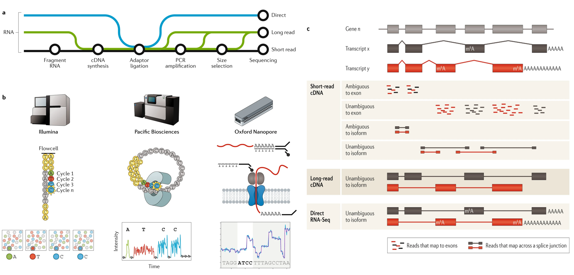
1.1 Advances in RNA-seq technologies
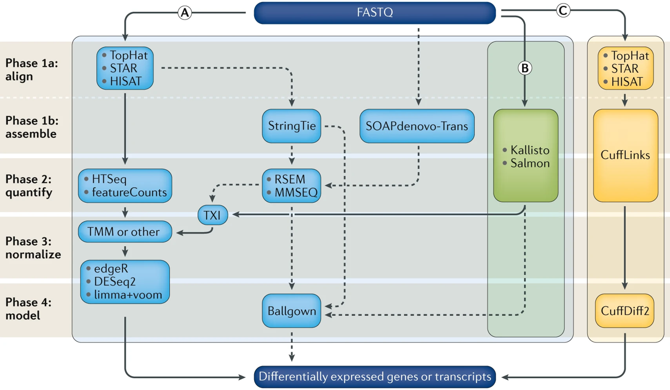
1.2 Different Pipelines
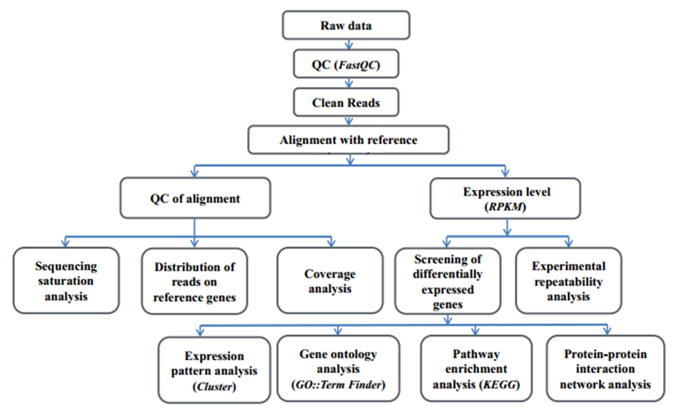
1.3 General Workflow
2. Prerequisite knowledge
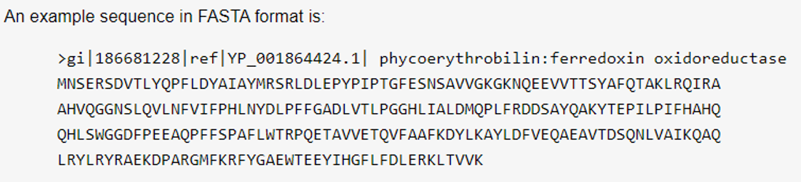
2.1 Data Format
- (1) FASTA
- (2) FASTQ
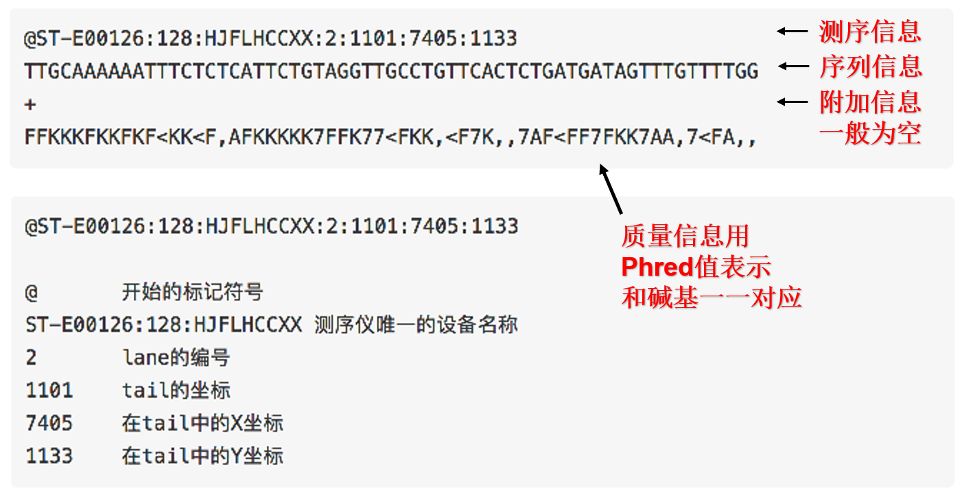
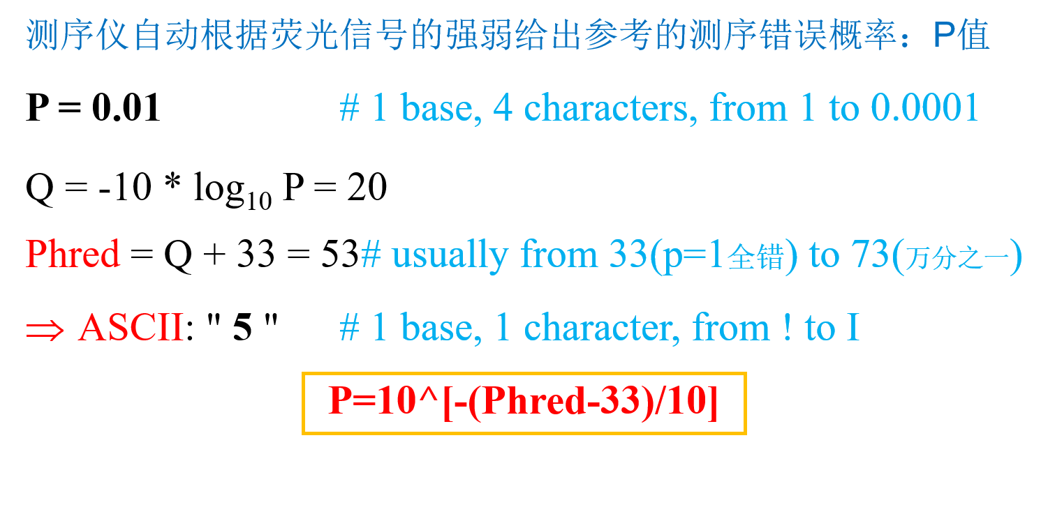
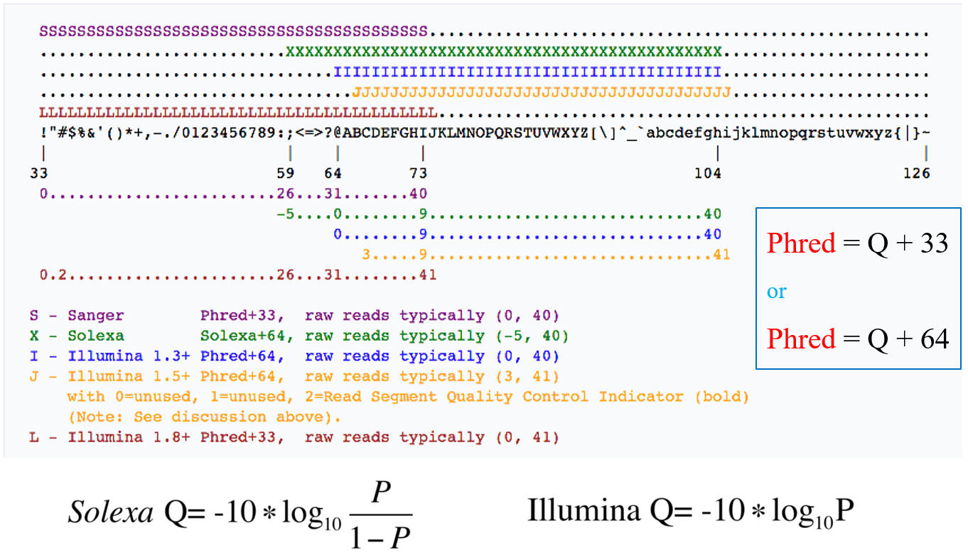
- (3) Phred quality scores
- (4) ASCII table
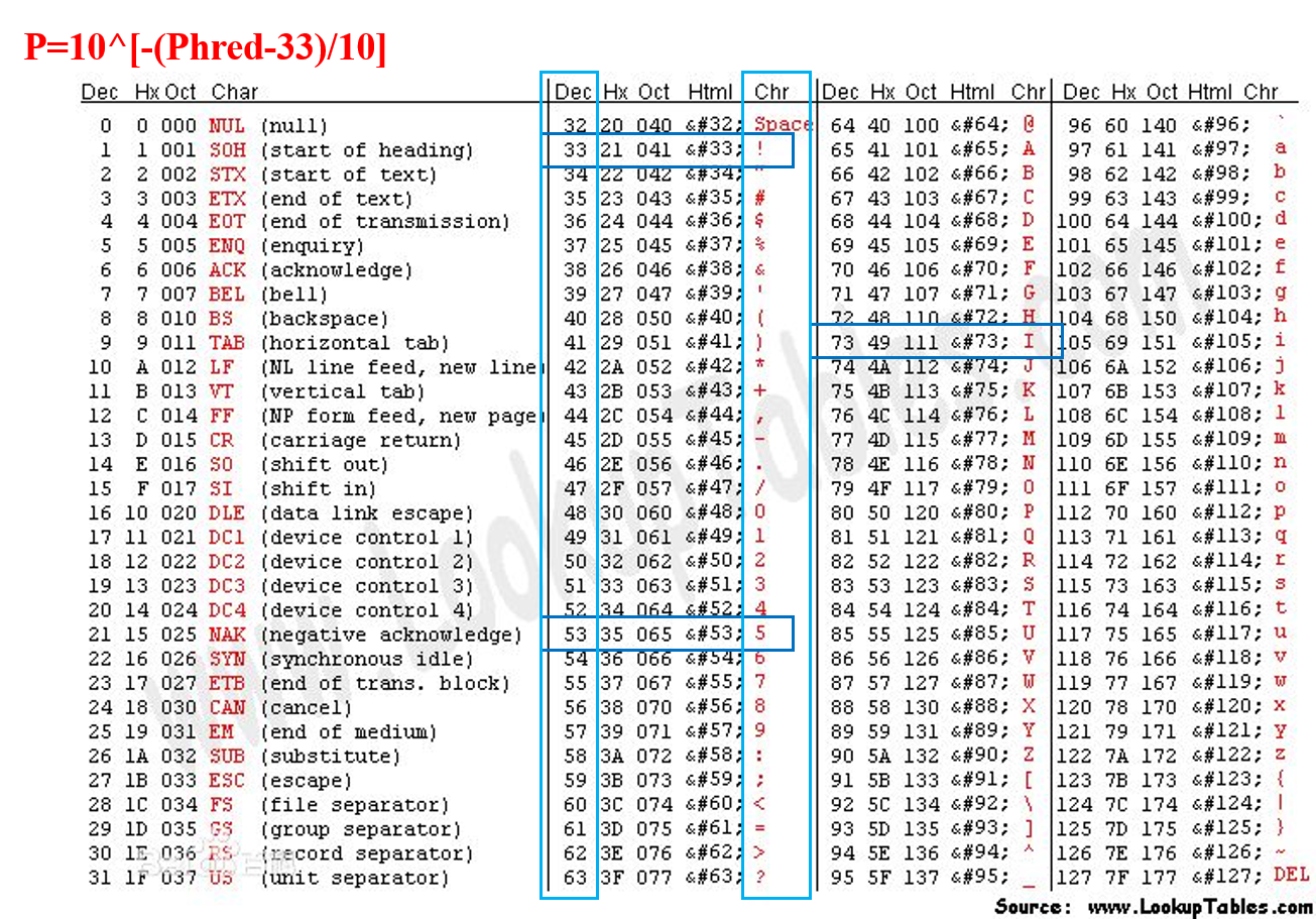
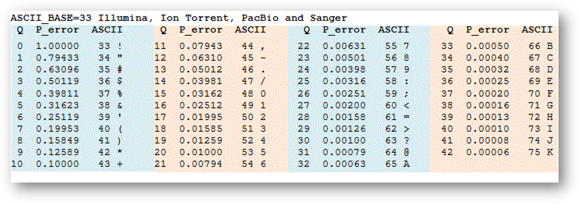
- (5) Quality scores
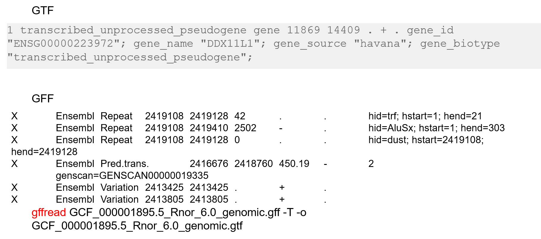
- (6) GTF & GFF
3. Data Sources
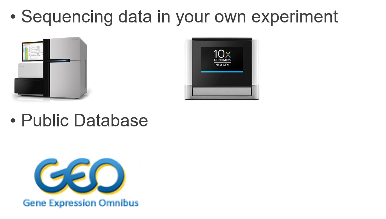
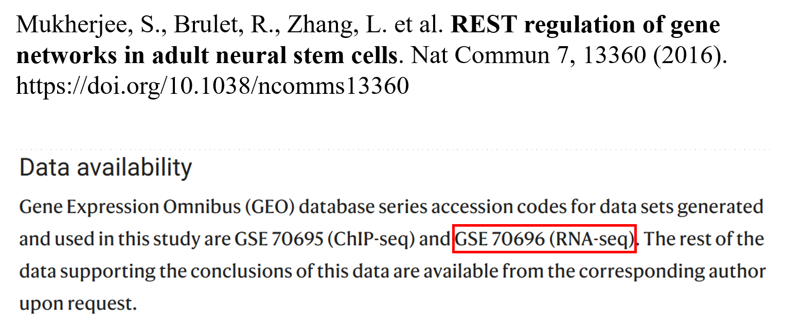
- (1) GEO (Gene Expression Omnibus)
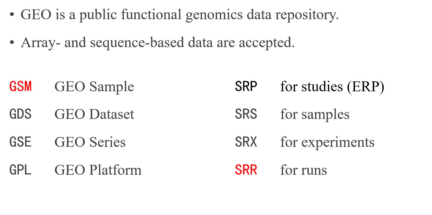
- (2) Get FASTQ file from GEO
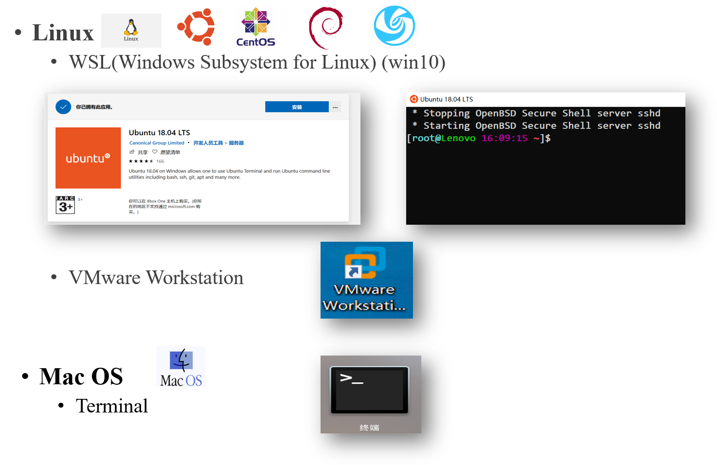
4. Computing Environment
二、准备工作
2.1 安装conda及相关软件
conda create -n scRNA-seq python=2
conda info --env
source activate scRNA-seq
conda install -y sra-tools cutadapt multiqc trim-galore subread hisat2
2.2 下载sra数据
#激活conda的scRNA-seq环境
conda activate scRNA-seq
cd /mnt/e/scRNA

#下载sra数据
mkdir raw_sra
wget -i download.txt

#检查数据完整性:md5值
#给文件生成md5值
md5sum *gz > md5.txt

#比对已有的md5值
md5sum -c md5.txt
2.3 sra文件转fastq文件
mkdir raw_fq
ls raw_sra/* | while read id; do (fastq-dump --gzip --split-e $id); done
三、数据质控
#查看qc前结果
for i in 'ls *gz';do fastqc $i;done
#或者
ls *gz | xargs -I [] echo 'nohup fastqc [] &'
#使用multiqc合并qc结果
multiqc ./
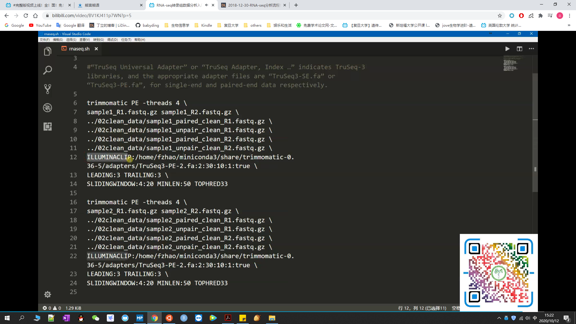
#用Trimmomatic过滤低质量序列
#注:接头序列的选择
#"Illumina Single End" / "Illumina Paired End": "TruSeq2-SE.fa" and "TruSeq3-PE.fa"
#"TruSeq Universal Adapter" / "TruSeq Adapter,Index...": "TruSeq3-SE.fa" and "TruSeq3-PE.fa"
#注:去接头参数的选择:true(双端测序选此) / false
#代码较长,如下图所示:
#查看qc后结果
for i in 'ls *gz';do fastqc $i;done
四、序列比对
(1)基于基因组比对(以染色体为单位):
- STAR
- Hisat2
(2)基于转录本比对(以转录本为单位):
- RSEM
4.1 STAR操作实例
(1)建立索引:
STAR --runThreadN 6 --runMode genomeGenerate \
--genomeDir arab_STAR_genome \
--genomeFastaFiles 00ref/TAIR10_Chr.all.fasta \
--sjdbGTFfile 00ref/Araport11_GFF3_genes_transposons.201606.gtf \
--sjdbOverhang 149 #预测可变剪接
(2)序列比对:
STAR --runThreadN 5 --genomeDir arab_STAR_genome \
--readFilesCommand zcat \
--readFilesIn 02clean_data/sample1_paired_clean_R1.fastq.gz \
02clean_data/sample1_paired_clean_R2.fastq.gz \
--outFileNamePrefix 03align_out/sample1_ \
--outSAMtype BAM SortedByCoordinate \
--outBAMsortingThreadN 5 \
--quantMode TranscriptomeSAM GeneCounts
4.2 Hisat2操作实例
(1)建立index:
mkdir reference
hisat2_extract_exons.py GRCm38.gtf  > exons.txt
hisat2_extract_splice_sites.py GRCm38.gtf > ss.txt
hisat2-build -p 8 --ss ss.txt --exon exons.txt GRCm38.fa GRCm38
(2)将fq文件比对至参考基因组:
index=/mnt/e/scRNA/reference/GRCm38
ls raw_fq/*gz | while read id; do (hisat2 -p 8 -x $index -U $id -S ${id%%.*}.hisat.sam); done

#sam格式转bam格式
mkdir align
mv raw_fq/*sam align/
ls *.sam | while read id; do (samtools sort -O bam -@ 5 -o $(basename ${id} ".sam").bam ${id});done

#为bam文件建立索引
ls *.bam | xargs -i samtools index {}
五、计算表达量
(1)STAR+RSEM:
- 输出结果可以选择转录本定量或者基因定量
- 定量单位包括feature count、FPKM、TPM
- 操作相对复杂
(2)STAR+HTSeq:
- 输出结果为原始read count
- 结果可用于差异表达分析
- 操作相对简单
(3)STAR+featureCounts:
- STAR+featureCounts = STAR+HTSeq升级版
- 安装:conda install subread
- 优点:快,非常快
(4)Kallisto (free-alignment):
- 速度快省内存
- 基于转录本定量
- 不产生bam文件不方便其他后续分析
5.1 STAR+RSEM演示
- 准备定量分析所需文件
- 利用STAR结果进行定量分析
# rsem prepare reference
rsem-prepare-reference --gtf 00ref/Araport11_GFF3_genes_transposons.201606.gtf \
00ref/TAIR10_Chr.all.fasta \
arab_RSEM/arab_rsem

rsem-calculate-expression --paired-end --no-bam-output \
--alignments -p 5 \
-q 03align_out/sample2_AlignedtoTranscriptome.out.bam \
arab_RSEM/arab_rsem \
04rsem_out/sample2_rsem

# htseq-count
htseq-count -r pos -m union -f bam -s no \
-q 03align_out/sample2Aligned.sortedByCoord.out.bam >
05htseq_out/sample2.htseq.out
5.2 Kallisto演示
- 利用转录本参考序列文件构建索引
- 进行无比对定量分析
# build index
kallisto index -i arab_kallisto ../arab_RSEM/arab_rsem.transcripts.fa

# count
kallisto quant -i arab_kallisto/arab_kallisto -o 05kallisto_out/sample2 \
02clean_data/sample2_paired_clean_R1.fastq.gz \
02clean_data/sample2_paired_clean_R2.fastq.gz
5.3 featureCounts演示
# 使用featureCounts进行定量
featureCounts -p -a ../00ref/Araport11_GFF3_genes_transposons.201606.gtf \
-o out_counts.txt -T 6 -t exon -g gene_id sample*_Aligned.sortedByCoord.out.bam
六、差异分析
6.1 表达定量结果转换为表达矩阵
- RSEM自带脚本
- 去除所有样本表达量全部为0的基因
mkdir 06deseq_out

# 构建表达矩阵
rsem-generate-data-matrix *_rsem.genes.results > output.matrix

# 删除未检测到表达的基因
awk 'BEGIN{printf "geneid\ta1\ta2\tb1\tb2\n"}{if($2+$3+$4+$5>0)print $0}' output.matrix > deseq2_input.txt
6.2 使用DESeq2进行差异表达分析
接下来在R-studio中操作:
# 读取文件
input_data <- read.table("deseq2_input.txt",header=TRUE,row.names=1)

# 取整
input_data <- round(input_data,digits=0)

# 准备工作
input_data <- as.matrix(input_data)
condition <- factor(c(rep("ctl",2),rep("exp",2)))
coldata <- data.frame(row.names=colnames(input_data),condition)
library(DESeq2)

# 构建deseq输入矩阵
dds <- DESeqDataSetFromMatrix(countData=input_data,colData=coldata,design=~condition)
# DESeq2进行差异分析
dds <- DESeq(dds)
# 提取结果
res <- results(dds)
summary(res)
res <- res[order(res$padj),]
resdata <- merge(as.data.frame(res),as.data.frame(counts(dds,normalized=TRUE)),by="row.names",sort=FALSE)
names(resdata)[1] <- "Gene"
6.3 可视化展示
# 可视化展示
maplot <- function(res,thresh=0.05,labelsig=TRUE, ...){
	with(res,plot(baseMean,log2FoldChange,pch=20,cex=0.5,log="x",...))
	with(subset(res,padj(thresh),points(baseMean,log2FoldChange,col="red",pch=20,cex=1.5)))
}
png("diffexor-maplot.png",1500,1000,pointsize=20)
maplot(resdata,main="MA Plot")
dev.off()


install.packages("ggrepel")
library(ggplot2)
library(ggrepel)

resdata$significant <- as.factor(resdata$padj<0.05 & abs(resdata$log2FoldChange)>1)
ggplot(data=resdata,aes(x=log2FoldChange,y=-log10(padj),color=significant))+geom_point()+ylim(0,8)+scale_color_manual(values=c("black","red"))+geom_hline(yintercept=-log10(0.05),lty=4,lwd=0.6,alpha=0.8)+
geom_vline(xintercept=c(1,-1),lty=4,lwd=0.6,alpha=0.8)+theme_bw()+theme(panel.grid.major=element_blank(),panel.grid.minor=element_blank(),axis.line=element_line(colour="black"))+itle="Volcanoplot",x="log2 (fold change)",y="-log10 (padj)")+plot.title=element_text(hjust=0.5)+ext_repel(data=subset(resdata,-log10(padj)>6),aes(label=Gene),col="black",alpha=0.8)
6.4 筛选上下调基因
# 筛选上下调基因
wc -l diffexpr-results.txt

awk '{if ($3>1 && $7<0.05) print $0}' diffexpr-results.txt | cut -f 1,2,4,7 > up.gene.txt

awk '{if ($3<-1 && $7<0.05) print $0}' diffexpr-results.txt | cut -f 1,2,4,7 > down.gene.txt
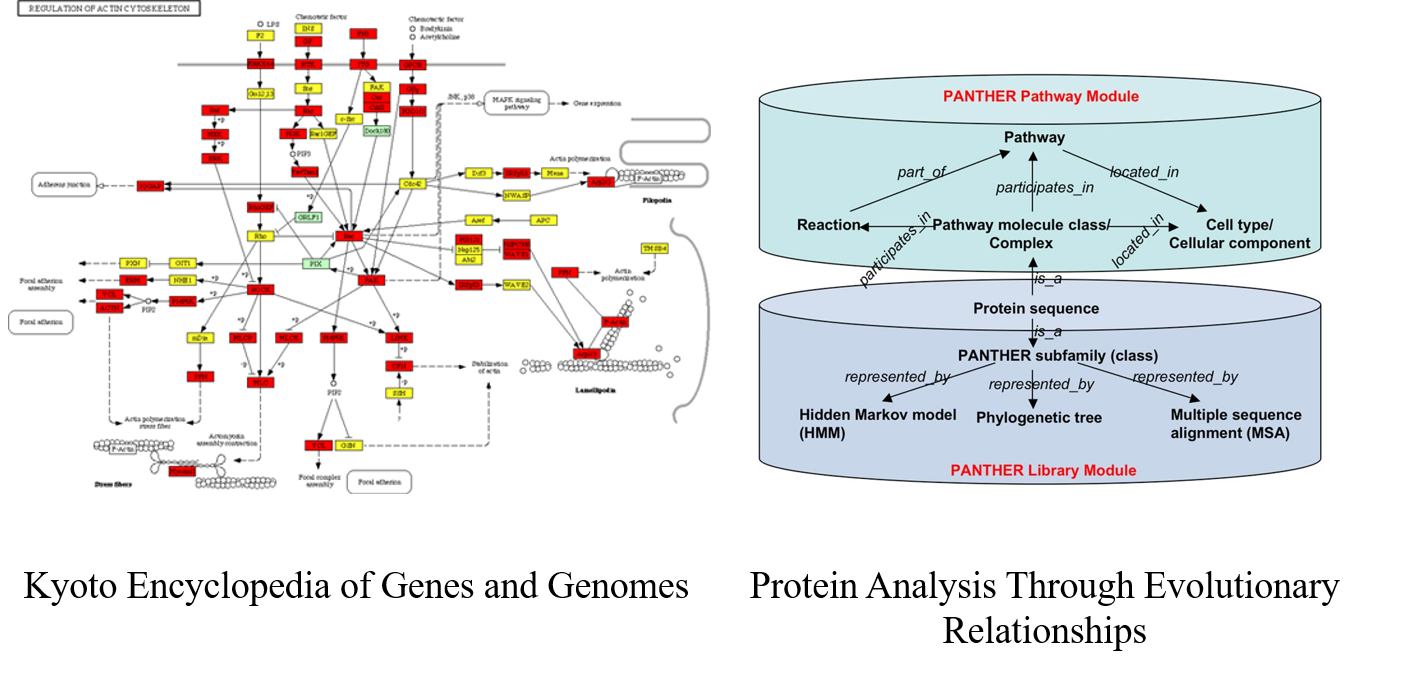
七、后续的富集分析
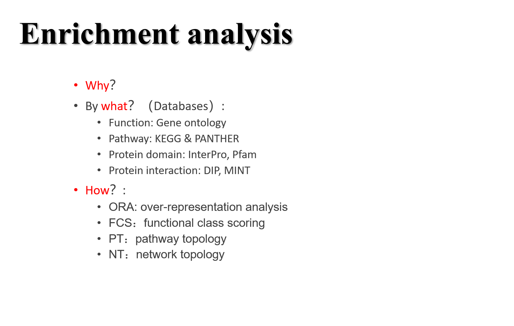
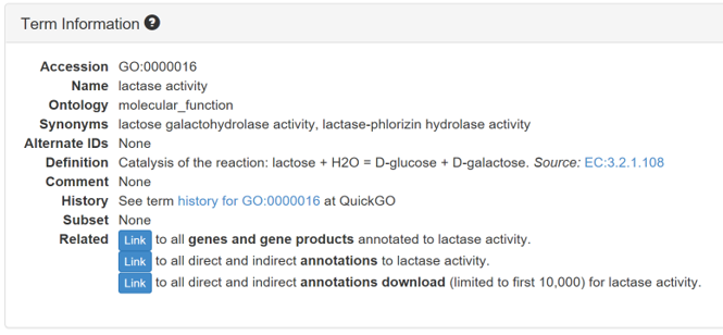
7.1 Gene ontology
Gene ontology (GO) is a major bioinformatics initiative to unify the representation of gene and gene product attributes across all species. The ontology covers three domains: cellular component, molecular function and biological process.
7.2 KEGG & PANTHER