资料来源:bioinfomics公众号
Seurat is an R package designed for QC, analysis, and exploration of single-cell RNA-seq data. Seurat aims to enable users to identify and interpret sources of heterogeneity from single-cell transcriptomic measurements, and to integrate diverse types of single-cell data.
0. 大纲
- 安装并加载所需的R包
- 构建Seurat对象
- 标准的数据预处理流程
- 数据的归一化
- 鉴定高可变基因(特征选择)
- 数据的标准化
- 进行PCA线性降维
- 选择PCA降维的维数用于后续的分析
- 细胞的聚类分群
- 非线性降维可视化(UMAP/tSNE)
- 鉴定不同类群之间的差异表达基因
- Marker基因的可视化
- 对聚类后的不同类群进行注释
1. 安装并加载所需的R包
本文所述的Seurat包都是基于3.0版本的,可以直接通过install.packages命令进行安装。
# 设置R包安装镜像
options(repos="https://mirrors.tuna.tsinghua.edu.cn/CRAN/")
install.packages('Seurat')
library(Seurat)
library(dplyr)
library(patchwork)
# 查看Seurat包的版本信息
packageVersion("Seurat")
2. 构建Seurat对象
本教程使用的是来自10X Genomics平台测序的外周血单核细胞(PBMC)数据集,这个数据集是用Illumina NextSeq 500平台进行测序的,里面包含了2,700个细胞的RNA-seq数据。
这个原始数据是用CellRanger软件进行基因表达定量处理的,最终生成了一个UMI的count矩阵。矩阵里的列是不同barcode指示的细胞,行是测序到的不同基因。接下来,我们将使用这个count矩阵创建Seurat对象。
# Load the PBMC dataset
pbmc.data <- Read10X(data.dir = "E:/Seurat_scRNA/00_raw_data/pbmc3k/filtered_gene_bc_matrices/hg19/")
# Initialize the Seurat object with the raw (non-normalized data).
# 初步过滤:每个细胞中至少检测到200个基因,每个基因至少在3个细胞中表达
pbmc <- CreateSeuratObject(counts = pbmc.data, project = "pbmc3k", min.cells = 3, min.features = 200)
pbmc
## An object of class Seurat
## 13714 features across 2700 samples within 1 assay
## Active assay: RNA (13714 features)
查看原始count矩阵的信息
# Lets examine a few genes in the first thirty cells
pbmc.data[c("CD3D", "TCL1A", "MS4A1"), 1:30]
## 3 x 30 sparse Matrix of class "dgCMatrix"
##
## CD3D  4 . 10 . . 1 2 3 1 . . 2 7 1 . . 1 3 . 2  3 . . . . . 3 4 1 5
## TCL1A . .  . . . . . . 1 . . . . . . . . . . .  . 1 . . . . . . . .
## MS4A1 . 6  . . . . . . 1 1 1 . . . . . . . . . 36 1 2 . . 2 . . . .
表达矩阵中的”.”表示某一基因在某一细胞中没有检测到表达,因为scRNA-seq的表达矩阵中会存在很多表达量为0的数据,Seurat会使用稀疏矩阵进行数据的存储,可以有效减少存储的内存。
3. 标准的数据预处理流程
Seurat可以对原始count矩阵进行质量控制,选择特定的质控条件进行细胞和基因的过滤,质控的一般指标包括:
- 每个细胞中能检测到的基因数目
1)低质量的细胞或空的droplets中能检测到的基因比较少
2)细胞doublets 或者 multiplets 中会检测到比较高数目的基因count数
- 每个细胞内能检测到的分子数
1)细胞内检测到的线粒体基因的比例
2)低质量/死细胞中通常会有比较高的线粒体污染
在Seurat中可以使用PercentageFeatureSet函数计算每个细胞中线粒体的含量:在人类参考基因中线粒体基因是以“MT-”开头的,而在小鼠中是以“mt-”开头的。
pbmc[["percent.mt"]] <- PercentageFeatureSet(pbmc, pattern = "^MT-")
# Show QC metrics for the first 5 cells
head(pbmc@meta.data, 5)
orig.ident    nCount_RNA  nFeature_RNA    percent.mt
AAACATACAACCAC    pbmc3k  2419    779 3.0177759
AAACATTGAGCTAC    pbmc3k  4903    1352    3.7935958
AAACATTGATCAGC    pbmc3k  3147    1129    0.8897363
AAACCGTGCTTCCG    pbmc3k  2639    960 1.7430845
AAACCGTGTATGCG    pbmc3k  980 521 1.2244898
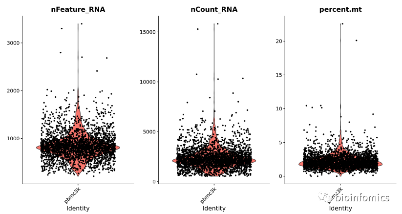
可视化QC指标,并用它们来过滤细胞:
1)将unique基因count数超过2500,或者小于200的细胞过滤掉
2)把线粒体含量超过5%以上的细胞过滤掉
# Visualize QC metrics as a violin plot
VlnPlot(pbmc, features = c("nFeature_RNA", "nCount_RNA", "percent.mt"), ncol = 3)
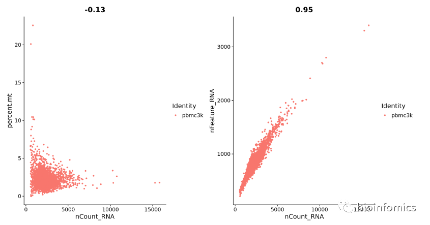
我们还可以使用FeatureScatter函数来对不同特征-特征之间的关系进行可视化
plot1 <- FeatureScatter(pbmc, feature1 = "nCount_RNA", feature2 = "percent.mt")
plot2 <- FeatureScatter(pbmc, feature1 = "nCount_RNA", feature2 = "nFeature_RNA")
plot1 + plot2
根据QC指标进行细胞和基因的过滤
pbmc <- subset(pbmc, subset = nFeature_RNA > 200 & nFeature_RNA < 2500 & percent.mt < 5)
4. 数据的归一化
默认情况下,Seurat使用global-scaling的归一化方法,称为“LogNormalize”,这种方法是利用总的表达量对每个细胞里的基因表达值进行归一化,乘以一个scale factor(默认值是10000),再用log转换一下。归一化后的数据存放在pbmc[[“RNA”]]@data里。
pbmc <- NormalizeData(pbmc, normalization.method = "LogNormalize", scale.factor = 10000)
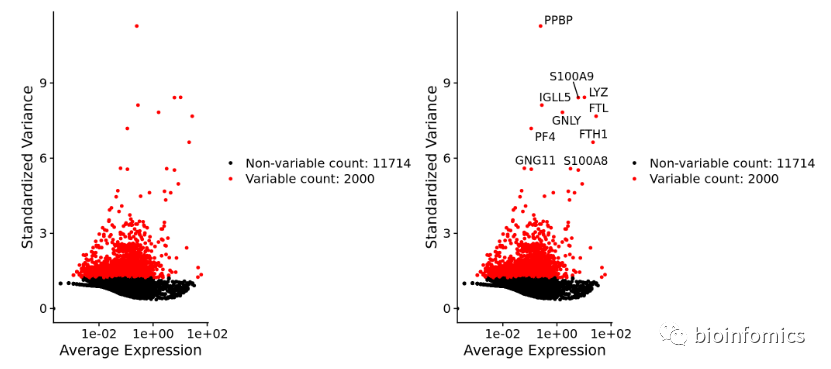
5. 鉴定高可变基因(特征选择)
Seurat使用FindVariableFeatures函数鉴定高可变基因,这些基因在PBMC不同细胞之间的表达量差异很大(在一些细胞中高表达,在另一些细胞中低表达)。默认情况下,会返回2,000个高可变基因用于下游的分析,如PCA等。
pbmc <- FindVariableFeatures(pbmc, selection.method = "vst", nfeatures = 2000)

# Identify the 10 most highly variable genes
top10 <- head(VariableFeatures(pbmc), 10)

# plot variable features with and without labels
plot1 <- VariableFeaturePlot(pbmc)
plot2 <- LabelPoints(plot = plot1, points = top10, repel = TRUE)
plot1 + plot2
6. 数据的标准化
Seurat使用ScaleData函数对归一化后的count矩阵进行一个线性的变换(“scaling”),将数据进行标准化:
1)shifting每个基因的表达,使细胞间的平均表达为0
2)scaling每个基因的表达,使细胞间的差异为1
ScaleData默认对之前鉴定到的2000个高可变基因进行标准化,也可以通过vars.to.regress参数指定其他的变量对数据进行标准化,表达矩阵进行scaling后,其结果存储在pbmc[[“RNA”]]@scale.data中。
pbmc <- ScaleData(pbmc)
all.genes <- rownames(pbmc)
pbmc <- ScaleData(pbmc, features = all.genes)
pbmc <- ScaleData(pbmc, vars.to.regress = "percent.mt")
7. 进行PCA线性降维
Seurat使用RunPCA函数对标准化后的表达矩阵进行PCA降维处理,默认情况下,只对前面选出的2000个高可变基因进行线性降维,也可以通过feature参数指定想要降维的数据集。
pbmc <- RunPCA(pbmc, features = VariableFeatures(object = pbmc))
# Examine and visualize PCA results a few different ways
print(pbmc[["pca"]], dims = 1:5, nfeatures = 5)
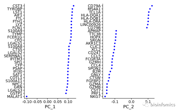
## PC_ 1
## Positive: CST3, TYROBP, LST1, AIF1, FTL
## Negative: MALAT1, LTB, IL32, IL7R, CD2
## PC_ 2
## Positive: CD79A, MS4A1, TCL1A, HLA-DQA1, HLA-DQB1
## Negative: NKG7, PRF1, CST7, GZMB, GZMA
## PC_ 3
## Positive: HLA-DQA1, CD79A, CD79B, HLA-DQB1, HLA-DPB1
## Negative: PPBP, PF4, SDPR, SPARC, GNG11
## PC_ 4
## Positive: HLA-DQA1, CD79B, CD79A, MS4A1, HLA-DQB1
## Negative: VIM, IL7R, S100A6, IL32, S100A8
## PC_ 5
## Positive: GZMB, NKG7, S100A8, FGFBP2, GNLY
## Negative: LTB, IL7R, CKB, VIM, MS4A7
Seurat可以使用VizDimReduction, DimPlot, 和DimHeatmap函数对PCA的结果进行可视化
VizDimLoadings(pbmc, dims = 1:2, reduction = "pca")
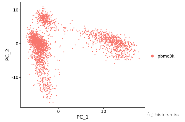
DimPlot(pbmc, reduction = "pca")
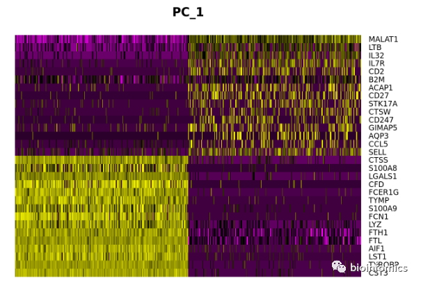
DimHeatmap(pbmc, dims = 1, cells = 500, balanced = TRUE)
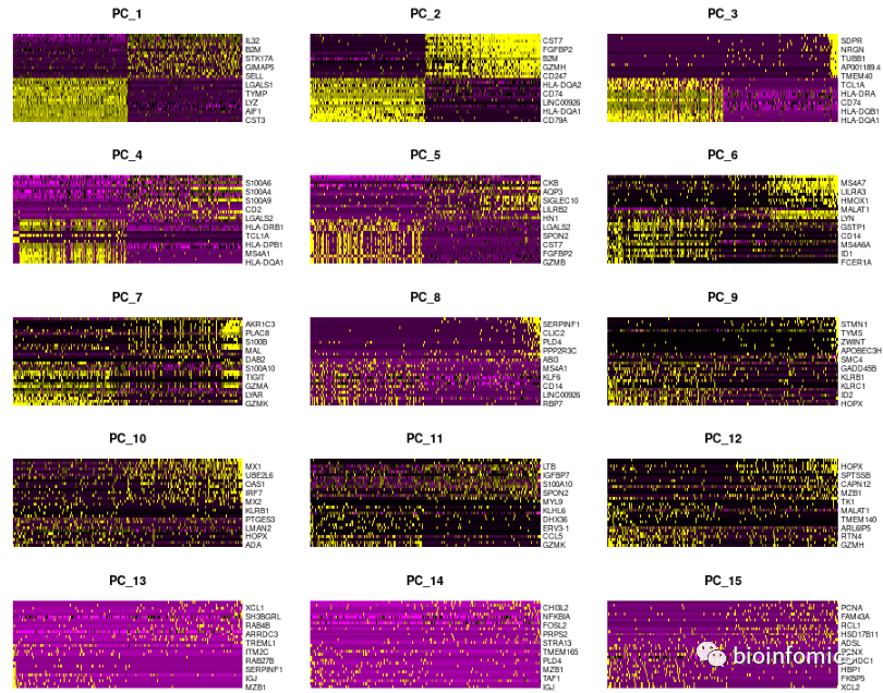
DimHeatmap(pbmc, dims = 1:15, cells = 500, balanced = TRUE)
8. 选择PCA降维的维数用于后续的分析
Seurat可以使用两种方法确定PCA降维的维数用于后续的聚类分析:
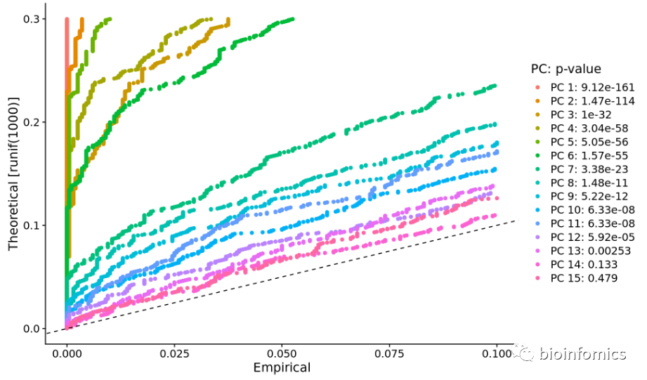
- (1)使用JackStrawPlot函数
使用JackStraw函数计算每个PC的P值的分布,显著的PC会有较低的p-value:
pbmc <- JackStraw(pbmc, num.replicate = 100)
pbmc <- ScoreJackStraw(pbmc, dims = 1:20)
# 使用JackStrawPlot函数进行可视化
JackStrawPlot(pbmc, dims = 1:15)
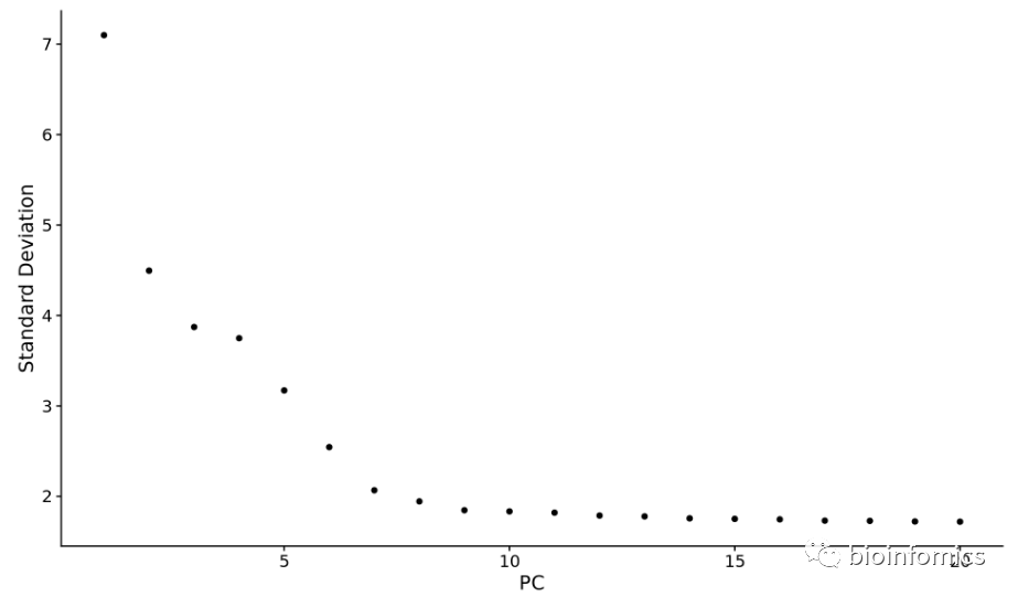
- (2)使用ElbowPlot函数
使用ElbowPlot函数查看在哪一个PC处出现平滑的挂点:
ElbowPlot(pbmc)
9. 细胞的聚类分群
Seurat使用图聚类的方法对降维后的表达数据进行聚类分群。
Briefly, these methods embed cells in a graph structure - for example a K-nearest neighbor (KNN) graph, with edges drawn between cells with similar feature expression patterns, and then attempt to partition this graph into highly interconnected ‘quasi-cliques’ or ‘communities’.
pbmc <- FindNeighbors(pbmc, dims = 1:10)
pbmc <- FindClusters(pbmc, resolution = 0.5)
## Modularity Optimizer version 1.3.0 by Ludo Waltman and Nees Jan van Eck
##
## Number of nodes: 2638
## Number of edges: 96033
##
## Running Louvain algorithm...
## Maximum modularity in 10 random starts: 0.8720
## Number of communities: 9
## Elapsed time: 0 seconds
# Look at cluster IDs of the first 5 cells
head(Idents(pbmc), 5)
## AAACATACAACCAC AAACATTGAGCTAC AAACATTGATCAGC AAACCGTGCTTCCG AAACCGTGTATGCG
##              1              3              1              2              6
## Levels: 0 1 2 3 4 5 6 7 8
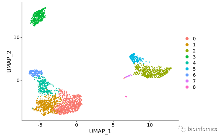
10. 非线性降维可视化(UMAP/tSNE)
Seurat offers several non-linear dimensional reduction techniques, such as tSNE and UMAP, to visualize and explore these datasets. The goal of these algorithms is to learn the underlying manifold of the data in order to place similar cells together in low-dimensional space.
# If you haven't installed UMAP, you can do so via reticulate::py_install(packages = 'umap-learn')
# UMAP降维可视化
pbmc <- RunUMAP(pbmc, dims = 1:10)
# note that you can set `label = TRUE` or use the LabelClusters function to help label individual clusters
DimPlot(pbmc, reduction = "umap")
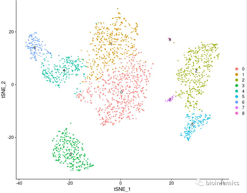
#tSNE降维可视化
pbmc <- RunTSNE(pbmc, dims = 1:10)
DimPlot(pbmc, reduction = "tsne", label = TRUE)
11. 鉴定不同类群之间的差异表达基因
Seurat使用FindMarkers和FindAllMarkers函数进行差异表达基因的筛选,可以通过test.use参数指定不同的差异表达基因筛选的方法。
# find all markers of cluster 1
cluster1.markers <- FindMarkers(pbmc, ident.1 = 1, min.pct = 0.25)
head(cluster1.markers, n = 5)

p_val    avg_logFC   pct.1   pct.2   p_val_adj
IL32    0   0.8373872   0.948   0.464   0
LTB    0   0.8921170   0.981   0.642   0
CD3D    0   0.6436286   0.919   0.431   0
IL7R    0   0.8147082   0.747   0.325   0
LDHB    0   0.6253110   0.950   0.613   0

# find all markers distinguishing cluster 5 from clusters 0 and 3
cluster5.markers <- FindMarkers(pbmc, ident.1 = 5, ident.2 = c(0, 3), min.pct = 0.25)
head(cluster5.markers, n = 5)

p_val    avg_logFC   pct.1   pct.2   p_val_adj
FCGR3A    0   2.963144    0.975   0.037   0
IFITM3    0   2.698187    0.975   0.046   0
CFD    0   2.362381    0.938   0.037   0
CD68    0   2.087366    0.926   0.036   0
RP11-290F20.3    0   1.886288    0.840   0.016   0

# find markers for every cluster compared to all remaining cells, report only the positive ones
pbmc.markers <- FindAllMarkers(pbmc, only.pos = TRUE, min.pct = 0.25, logfc.threshold = 0.25)
pbmc.markers %>% group_by(cluster) %>% top_n(n = 2, wt = avg_logFC)

p_val    avg_logFC   pct.1   pct.2   p_val_adj   cluster gene
0    0.7300635   0.901   0.594   0   0   LDHB
0    0.9219135   0.436   0.110   0   0   CCR7
0    0.8921170   0.981   0.642   0   1   LTB
0    0.8586034   0.422   0.110   0   1   AQP3
0    3.8608733   0.996   0.215   0   2   S100A9
0    3.7966403   0.975   0.121   0   2   S100A8
0    2.9875833   0.936   0.041   0   3   CD79A
0    2.4894932   0.622   0.022   0   3   TCL1A
0    2.1220555   0.985   0.240   0   4   CCL5
0    2.0461687   0.587   0.059   0   4   GZMK
0    2.2954931   0.975   0.134   0   5   FCGR3A
0    2.1388125   1.000   0.315   0   5   LST1
0    3.3462278   0.961   0.068   0   6   GZMB
0    3.6898996   0.961   0.131   0   6   GNLY
0    2.6832771   0.812   0.011   0   7   FCER1A
0    1.9924275   1.000   0.513   0   7   HLA-DPB1
0    5.0207262   1.000   0.010   0   8   PF4
0    5.9443347   1.000   0.024   0   8   PPBP
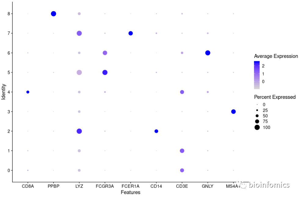
12. Marker基因的可视化
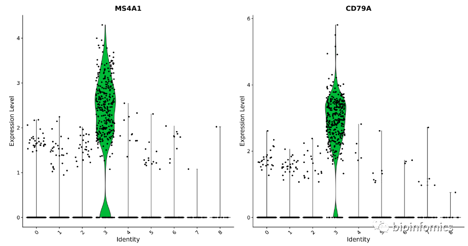
Seurat可以使用VlnPlot,FeaturePlot,RidgePlot,DotPlot和DoHeatmap等函数对marker基因的表达进行可视化
VlnPlot(pbmc, features = c("MS4A1", "CD79A"))
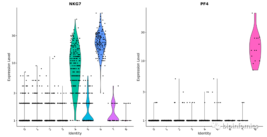
# you can plot raw counts as well
VlnPlot(pbmc, features = c("NKG7", "PF4"), slot = "counts", log = TRUE)
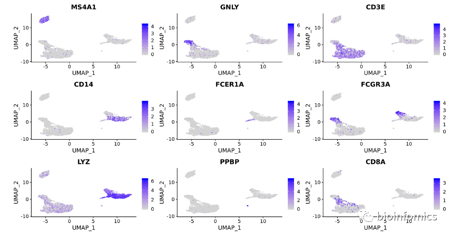
FeaturePlot(pbmc, features = c("MS4A1", "GNLY", "CD3E", "CD14", "FCER1A", "FCGR3A", "LYZ", "PPBP", "CD8A"))
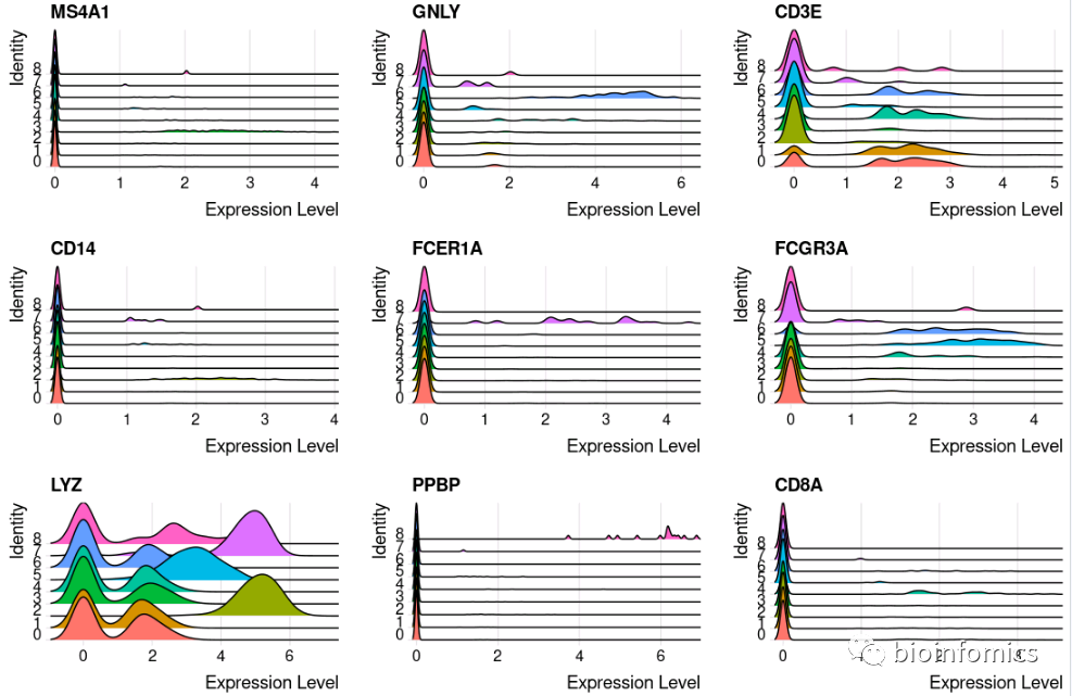
RidgePlot(pbmc, features = c("MS4A1", "GNLY", "CD3E", "CD14", "FCER1A", "FCGR3A", "LYZ", "PPBP", "CD8A"))
DotPlot(pbmc, features = c("MS4A1", "GNLY", "CD3E", "CD14", "FCER1A", "FCGR3A", "LYZ", "PPBP", "CD8A"))
top10 <- pbmc.markers %>% group_by(cluster) %>% top_n(n = 10, wt = avg_logFC)
DoHeatmap(pbmc, features = top10$gene) + NoLegend()

13. 对聚类后的不同类群进行注释
我们可以基于已有的生物学知识,根据一些特异的marker基因不细胞类群进行注释
Cluster ID    Markers Cell Type
IL7R, CCR7  Naive CD4+ T
IL7R, S100A4    Memory CD4+
CD14, LYZ   CD14+ Mono
MS4A1   B
CD8A    CD8+ T
FCGR3A, MS4A7   FCGR3A+ Mono
GNLY, NKG7  NK
FCER1A, CST3    DC
PPBP    Platelet
以上是根据PBMC中不同细胞类群的一些marker基因进行细胞分群注释的结果
# 根据marker基因进行分群注释
new.cluster.ids <- c("Naive CD4 T", "Memory CD4 T", "CD14+ Mono", "B", "CD8 T", "FCGR3A+ Mono", "NK", "DC", "Platelet")
names(new.cluster.ids) <- levels(pbmc)
# 细胞分群的重命名
pbmc <- RenameIdents(pbmc, new.cluster.ids)
DimPlot(pbmc, reduction = "umap", label = TRUE, pt.size = 0.5) + NoLegend()

# 保存分析的结果
saveRDS(pbmc, file = "../output/pbmc3k_final.rds")
sessionInfo()

R version 3.6.0 (2019-04-26)
Platform: x86_64-redhat-linux-gnu (64-bit)
Running under: CentOS Linux 7 (Core)

Matrix products: default
BLAS/LAPACK: /usr/lib64/R/lib/libRblas.so

locale:
[1] LC_CTYPE=en_US.UTF-8       LC_NUMERIC=C
[3] LC_TIME=en_US.UTF-8        LC_COLLATE=en_US.UTF-8
[5] LC_MONETARY=en_US.UTF-8    LC_MESSAGES=en_US.UTF-8
[7] LC_PAPER=en_US.UTF-8       LC_NAME=C
[9] LC_ADDRESS=C               LC_TELEPHONE=C
[11] LC_MEASUREMENT=en_US.UTF-8 LC_IDENTIFICATION=C

attached base packages:
[1] splines   parallel  stats4    grid      stats     graphics  grDevices
[8] utils     datasets  methods   base

other attached packages:
[1] loomR_0.2.1.9000            hdf5r_1.3.1
[3] R6_2.4.0                    mclust_5.4.5
[5] garnett_0.1.16              org.Hs.eg.db_3.8.2
[7] AnnotationDbi_1.46.0        pagedown_0.9.1
[9] devtools_2.1.0              usethis_1.5.1
[11] celaref_1.2.0               scran_1.12.1
[13] scRNAseq_1.10.0             FLOWMAPR_1.2.0
[15] Seurat_3.1.4.9902           sctransform_0.2.0
[17] patchwork_0.0.1             cowplot_1.0.0
[19] DT_0.12                     RColorBrewer_1.1-2
[21] shinydashboard_0.7.1        ggsci_2.9
[23] shiny_1.3.2                 stxBrain.SeuratData_0.1.1
[25] pbmcsca.SeuratData_3.0.0    panc8.SeuratData_3.0.2
[27] SeuratData_0.2.1            doParallel_1.0.14
[29] iterators_1.0.12            binless_0.15.1
[31] RcppEigen_0.3.3.5.0         foreach_1.4.7
[33] scales_1.0.0                dplyr_0.8.3
[35] pagoda2_0.1.0               harmony_1.0
[37] Rcpp_1.0.2                  conos_1.1.2