Here I provide a short description of the different steps of scRNAseq analysis using Seurat software (based on R). The dataset used in the analysis is GSE130973, the related paper is “Single-cell transcriptomes of the aging human skin reveal loss of fibroblast priming”.
1.The introduction of scRNA-seq:
1.1 Single-cell RNA-seq workflow
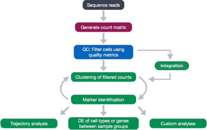
The scRNA-seq method will determine how to parse the barcodes and UMIs from the sequencing reads. So, although a few of the specific steps will slightly differ, the overall workflow will generally follow the same steps regardless of method. The general workflow is shown below:
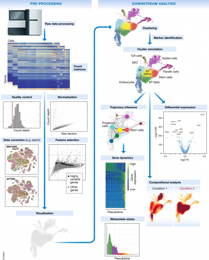
The steps of the workflow are:
- Generation of the count matrix (method-specific steps): formating reads, demultiplexing samples, mapping and quantification
- Quality control of the raw counts: filtering of poor quality cells
- Clustering of filtered counts: clustering cells based on similarities in transcriptional activity (cell types = different clusters)
- Marker identification: identifying gene markers for each cluster
- Optional downstream steps
1.2 The description of count data
Regardless of the technology or pipeline used to process our single-cell RNA-seq sequence data, the output will generally be the same. That is, for each individual sample we will have the following three files:
- a file with the cell IDs, representing all cells quantified
- a file with the gene IDs, representing all genes quantified
- a matrix of counts per gene for every cell
1.2.1 barcodes.tsv
This is a text file which contains all cellular barcodes present for that sample. Barcodes are listed in the order of data presented in the matrix file (i.e. these are the column names).
1.2.2 features.tsv
This is a text file which contains the identifiers of the quantified genes. The source of the identifier can vary depending on what reference (i.e. Ensembl, NCBI, UCSC) you use in the quantification methods, but most often these are official gene symbols. The order of these genes corresponds to the order of the rows in the matrix file (i.e. these are the row names).
1.2.3 matrix.mtx
This is a text file which contains a matrix of count values. The rows are associated with the gene IDs above and columns correspond to the cellular barcodes. Note that there are many zero values in this matrix.
More specifically, the first column is the ID of the gene, which is used for corresponding conversion with features.tsv; the second column is the cellular barcodes, which matches barcodes.tsv; the third column is the expression level of the gene TPM.
The summary of File format
| File | Format |
|---|---|
| barcodes.tsv (1 column) | cellular barcode |
| genes.tsv (2 columns) | ensembl ID; gene symbol |
| matrix.mtx (3 columns) | gene ID; cellular barcode; count value |
2.Quality Control for 5 Fribroblast 10x samples individually
2.1 Downloading the count matrix data
Firstly, we download the count matrix file from NCBI, which contains a set of 5 Fribroblast 10x datasets from 3 young individuals and 2 old individuals. This dataset is available on GEO (GSE130973). From the figure 6 we can see, the count matrix data of all five samples have been merged. The complete count matrix file contains a total of three sub-files: barcodes.tsv, genes.tsv and matrix.mtx.
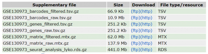
1.2 Loading the data into a seurat object
Loading the three count matrix data into R requires us to use functions that allow us to efficiently combine these three files into a single count matrix. However, instead of creating a regular matrix data structure, the functions we will use create a sparse matrix to improve the amount of space, memory and CPU required to work with our huge count matrix.
Here, we will use Read10X() function from the Seurat package and use the Cell Ranger output directory as input (contains barcodes.tsv, genes.tsv and matrix.mtx). In this way individual files do not need to be loaded in, instead the function will load and combine them into a sparse matrix for us. We will be using this function to load in our data!
sdata <- Read10X(data.dir = "./01_raw_data/")
alldata <- CreateSeuratObject(counts = sdata)

alldata@meta.data$age <- rep(c("young1","young2","old1","old2","old3"), times=c(3130,2829,3332,2222,4549))
alldata@meta.data$type <- rep(c("young","old"), times=c(5959,10103))
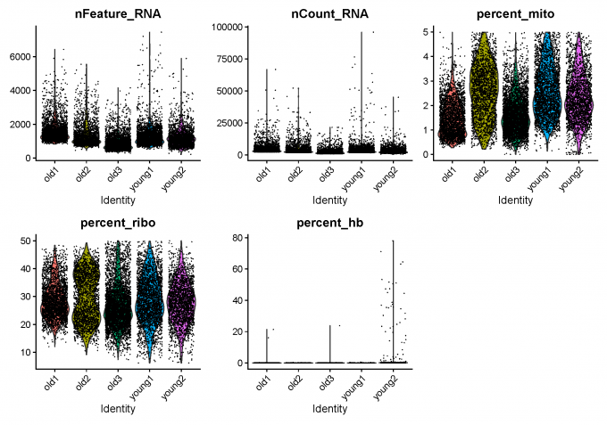
1.3 Calculate QC
I calculate some quality metrics using PercentageFeatureSet() and then do the detection-based filtering.
# Percentage mitocondrial genes
alldata <- PercentageFeatureSet(alldata, "^MT-", col.name = "percent_mito")

# Percentage ribosomal genes
alldata <- PercentageFeatureSet(alldata, "^RP[SL]", col.name = "percent_ribo")
1.4 Detection-based filtering
Initially, I filter cells with low amount of reads as well as genes that are present in at least a certain amount of cells. I only consider cells with at least 200 detected genes and less than 7500 genes. Pkus, genes need to be expressed in at least 3 cells.
selected_c <- WhichCells(alldata, expression = nFeature_RNA > 200 & nFeature_RNA < 7500)
selected_f <- rownames(alldata)[Matrix::rowSums(alldata) > 3]
data.filt <- subset(alldata, features = selected_f, cells = selected_c)
1.5 Mito/Ribo filtering
Then, I remove cells with high proportion of mitochondrial and low proportion ofribosomal reads.
selected_mito <- WhichCells(data.filt, expression = percent_mito < 5)
selected_ribo <- WhichCells(data.filt, expression = percent_ribo > 5 & percent_ribo < 50)
data.filt <- subset(data.filt, cells = selected_mito)
data.filt <- subset(data.filt, cells = selected_ribo)
1.6 Filter mitochondrial and MALAT1 genes
As the level of expression of mitochondrial and MALAT1 genes are judged as mainly technical, it can be wise to remove them from the dataset bofore any further analysis.
data.filt <- data.filt[!grepl("MALAT1", rownames(data.filt)), ]
data.filt <- data.filt[!grepl("^MT-", rownames(data.filt)), ]
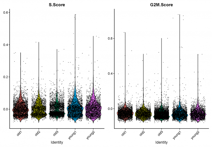
1.7 Calculate cell-cycle scores
data.filt = NormalizeData(data.filt)
data.filt <- CellCycleScoring(object = data.filt, g2m.features = cc.genes$g2m.genes, s.features = cc.genes$s.genes)
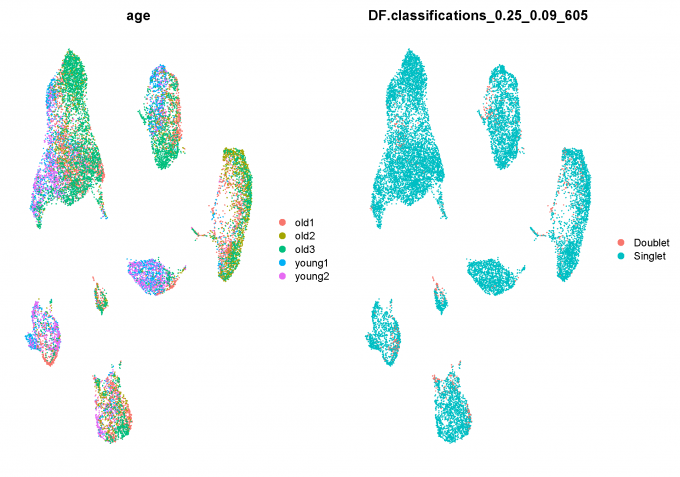
1.8 Predict doublets and delete them
Here, I use DoubletFinder package to predict doublet cells.
suppressMessages(require(DoubletFinder))
data.filt = FindVariableFeatures(data.filt, verbose = F)
data.filt = ScaleData(data.filt, vars.to.regress = c("nFeature_RNA", "percent_mito"),
                      verbose = F)
data.filt = RunPCA(data.filt, verbose = F, npcs = 20)
data.filt = RunUMAP(data.filt, dims = 1:10, verbose = F)
nExp <- round(ncol(data.filt) * 0.04)
data.filt <- doubletFinder_v3(data.filt, pN = 0.25, pK = 0.09, nExp = nExp, PCs = 1:10)

data.filt = data.filt[, data.filt@meta.data[, DF.name] == "Singlet"]
1.9 Clean scRNA-seq Data after QC
Step 2: Integrate 5 datasets and do dimensionality reduction
2.1 Data integration
Seurat uses the CCA method to do the integration of Single Cell Data.
alldata.anchors <- FindIntegrationAnchors(object.list = alldata.list, dims = 1:30,
    reduction = "cca")
alldata.int <- IntegrateData(anchorset = alldata.anchors, dims = 1:30, new.assay.name = "CCA")
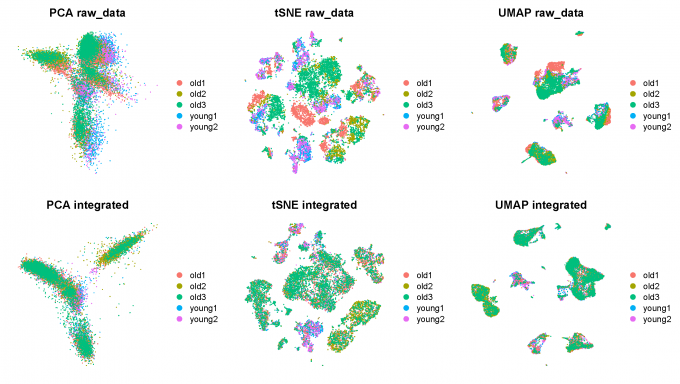
2.2 Dimensionality reduction
After running IntegrateData, the Seurat object will contain a new Assay with the batch-corrected expression matrix. I then use this new integrated matrix for downstream analysis and visualization.
I scale the integrated data, run PCA, and visualize the results with UMAP and TSNE. The integrated datasets cluster by cell type, instead of by technology.
alldata.int <- ScaleData(alldata.int, verbose = FALSE)
alldata.int <- RunPCA(alldata.int, npcs = 30, verbose = FALSE)
alldata.int <- RunUMAP(alldata.int, dims = 1:30)
alldata.int <- RunTSNE(alldata.int, dims = 1:30)
Step 3: Clustering
In this step, I use the integrated PCA to perform the clustering. I use three methods to perform clustering (kNN-graph-clustering, K-means clustering and Hierarchical clustering).
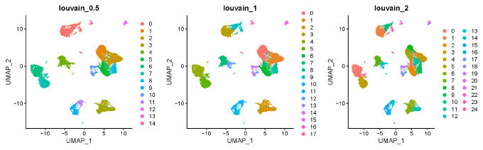
3.1 Clustering method 1: kNN-graph-clustering
alldata <- FindNeighbors(alldata, dims = 1:30, k.param = 60, prune.SNN = 1/15)
# Clustering with louvain (algorithm 1)
for (res in c(0.1, 0.25, 0.5, 1, 1.5, 2)) {
alldata <- FindClusters(alldata, graph.name = "CCA_snn", resolution = res, algorithm = 1)
}
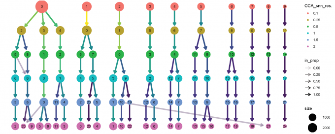
# Use the clustree package to visualize how cells are distributed between clusters depending on resolution.
clustree(alldata@meta.data, prefix = "CCA_snn_res.")
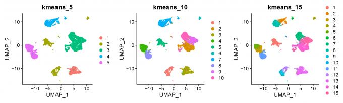
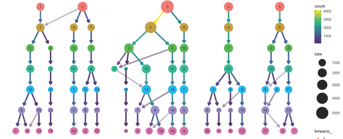
3.2 Clustering method 2: K-means clustering
for (k in c(5, 7, 10, 12, 15, 17, 20)) {
    alldata@meta.data[, paste0("kmeans_", k)] <- kmeans(x = alldata@reductions[["pca"]]@cell.embeddings,
        centers = k, nstart = 100)$cluster
}

clustree(alldata@meta.data, prefix = "kmeans_")
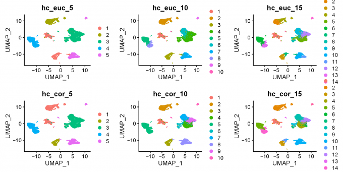
3.3 Clustering method 3: Hierarchical clustering
d <- dist(alldata@reductions[["pca"]]@cell.embeddings, method = "euclidean")

# Compute sample correlations
sample_cor <- cor(Matrix::t(alldata@reductions[["pca"]]@cell.embeddings))

# Transform the scale from correlations
sample_cor <- (1 - sample_cor)/2

# Convert it to a distance object
d2 <- as.dist(sample_cor)

# euclidean
h_euclidean <- hclust(d, method = "ward.D2")

# correlation
h_correlation <- hclust(d2, method = "ward.D2")

#euclidean distance
alldata$hc_euclidean_5 <- cutree(h_euclidean,k = 5)
alldata$hc_euclidean_10 <- cutree(h_euclidean,k = 10)
alldata$hc_euclidean_15 <- cutree(h_euclidean,k = 15)

#correlation distance
alldata$hc_corelation_5 <- cutree(h_correlation,k = 5)
alldata$hc_corelation_10 <- cutree(h_correlation,k = 10)
alldata$hc_corelation_15 <- cutree(h_correlation,k = 15)
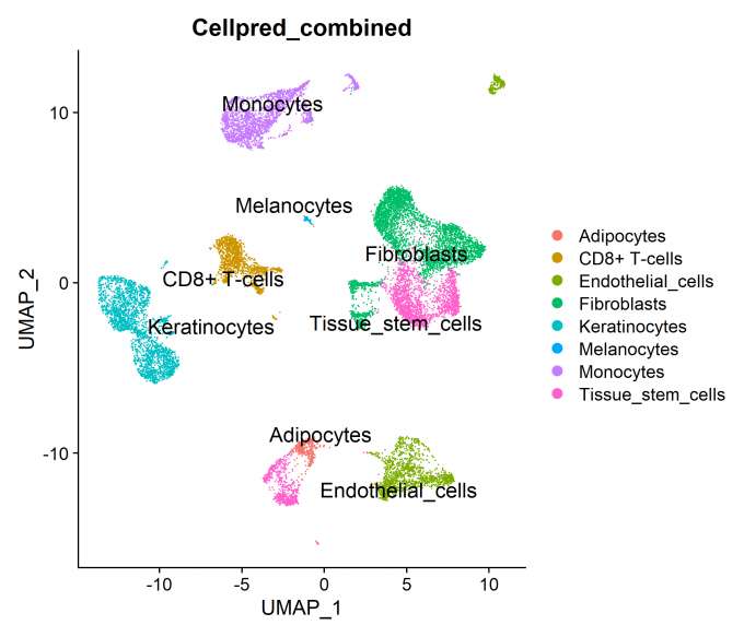
Step 4: Celltype prediction
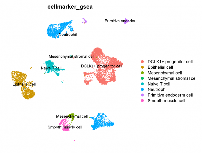
In this step, I set the identity as louvain with resolution 0.5 and use two methods to predict celltype: (1) SingleR software combining HumanPrimaryCellAtlas and BlueprintEncode database; (2) Gene set enrichment (GSEA) analysis combining CellMarker database, this method is based on the DEGs of each cluster.
4.1 SingleR + reference database (HCPA/BP)
4.2 GSEA analysis + CellMarker database
Step 5: Neuron marker identification